~ add a pull down select menu in google sheet ~

Example:

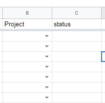
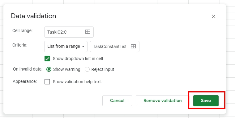
Added a new sheet and put the push down list on it

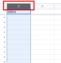
First, select the whole row

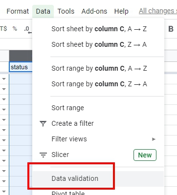
Data>Data validation

Change the Cell Range to C2:C
which means the formula will excluded the row 1(header)

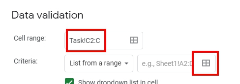
Click on Criteria box

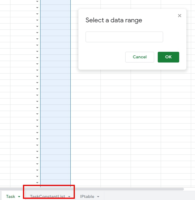
Choose the list sheet

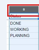
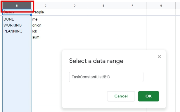
Highlight the whole row which you want to able to select in the pull down menu, and changed to TaskConstantList!B2:B to skip the header